USGS streamgages: bounded discovery and mapping

The USGS waterdata OGC API is a clean, real-world EDR endpoint with one collection (daily-edr) that exposes every USGS station’s daily-value time series. It’s a good target for learning edr4r because the API surface is small and the data is familiar (stream gauges).

This vignette walks through a typical streamgage exploration: discover what’s on offer, follow every advertised location page inside a small northern North Carolina Piedmont study area, pull recent streamflow for each station, and render an interactive map. The displayed results were precomputed from the live USGS endpoint so package checks remain offline.

1. Connect and discover collections

library(edr4r)
library(ggplot2)

usgs <- edr_client("https://api.waterdata.usgs.gov/ogcapi/beta")
edr_collections(usgs)[, c("id", "title", "data_queries")]
#> # A tibble: 1 × 3
#>   id        title                                           data_queries
#>   <chr>     <chr>                                           <list>      
#> 1 daily-edr Daily values environmental data retrieval (EDR) <chr [1]>

USGS exposes a single collection, daily-edr. The data_queries column tells us what query verbs it supports:

edr_collections(usgs)$data_queries[[1]]
#> [1] "locations"

Just locations. No cube, no area, no position. That matters: edr_explore() will fall back to per-station fetches instead of one bulk call. For a handful of gauges that’s fine; for thousands it would be slow. The WWDH rise-edr collection in vignette("getting-started") shows the bulk-fetch path against a richer server.

Discovering parameters

edr_parameters() reads the parameter_names block from the collection document – but USGS doesn’t populate it. Use edr_queryables() instead to see what filter properties the server exposes:

q <- edr_queryables(usgs, "daily-edr")
names(q$properties)
#>  [1] "geometry"                      "id"                           
#>  [3] "unit_of_measure"               "parameter_name"               
#>  [5] "parameter_code"                "statistic_id"                 
#>  [7] "hydrologic_unit_code"          "state_name"                   
#>  [9] "last_modified"                 "begin"                        
#> [11] "end"                           "computation_period_identifier"
#> [13] "computation_identifier"        "thresholds"                   
#> [15] "sublocation_identifier"        "primary"                      
#> [17] "monitoring_location_id"        "web_description"              
#> [19] "parameter_description"         "parent_time_series_id"

parameter_code is the filter you’d pass as parameter_name = in a query. USGS uses the standard NWIS parameter codes – a few common ones for streamgages:

Code	Meaning	Unit
`00060`	Discharge (streamflow)	ft³/s
`00065`	Gage height (stage)	ft
`00010`	Water temperature	°C
`00400`	pH	std units
`00095`	Specific conductance	µS/cm

The rest of this vignette uses 00060 – daily mean streamflow.

2. Find streamgages in a bounded study area

A compact box around several Tar River tributaries keeps this example small while still forcing more than one server page:

piedmont_bbox <- c(-78.60, 36.04, -78.28, 36.22)
#                    minx   miny    maxx   maxy

USGS paginates its location index with an opaque cursor. Opt into bounded pagination to make “every gauge” explicit; limit is the page size, while the two client-side caps guard the total pull. With sf installed the combined response is an sf object with one point per gauge:

gauges <- edr_locations(
  usgs, "daily-edr",
  bbox = piedmont_bbox,
  limit = 2,
  paginate = TRUE,
  max_pages = 10,
  max_features = 20
)
nrow(gauges)
#> [1] 5

gauges[, c("id", "monitoring_location_name", "county_name", "drainage_area")]
#> Simple feature collection with 5 features and 4 fields
#> Geometry type: POINT
#> Dimension:     XY
#> Bounding box:  xmin: -78.58306 ymin: 36.05404 xmax: -78.29611 ymax: 36.2132
#> Geodetic CRS:  WGS 84
#> # A tibble: 5 × 5
#>    id              monitoring_location_name            county_name drainage_area
#>    <chr>           <chr>                               <chr>               <dbl>
#>  1 USGS-02081500   TAR RIVER NEAR TAR RIVER, NC        Granville …        167   
#>  2 USGS-02081740   TAR RIVER AT LOUISBURG, NC          Franklin C…        429   
#>  3 USGS-02081747   TAR R AT US 401 AT LOUISBURG, NC    Franklin C…        427   
#>  4 USGS-02081800   CEDAR CREEK NEAR LOUISBURG, NC      Franklin C…         47.8 
#>  5 USGS-0208273070 DEVILS CRADLE C AT NC 39 NR KEARNE… Franklin C…          2.89
#> # ℹ 1 more variable: geometry <POINT [°]>

Each gauges$id is in the form "USGS-02087500" (agency code + the familiar 8-digit NWIS site number). That’s what you pass back as location_id = to a query.

3. Pull streamflow for one station

A USGS quirk to flag up front: when you ask for a specific station with edr_location(), the server ignores the datetime interval and just returns the most recent limit records (limit defaults to 10). To get five months of daily data, pass a limit that comfortably covers the window – say 200 days – and filter to the target window client-side.

example_id   <- gauges$id[[1]]
example_name <- gauges$monitoring_location_name[[1]]

resp <- edr_location(
  usgs, "daily-edr",
  location_id    = example_id,
  parameter_name = "00060",
  limit          = 200
)
df <- covjson_to_tibble(resp)

# Filter to the Jan–May 2026 window we care about
df_jan_may <- df[df$datetime >= as.POSIXct("2026-01-01", tz = "UTC") &
                 df$datetime <= as.POSIXct("2026-05-31", tz = "UTC"), ]
head(df_jan_may[, c("datetime", "value", "unit")])
#> # A tibble: 6 × 3
#>   datetime            value unit 
#>   <dttm>              <dbl> <chr>
#> 1 2026-05-31 00:00:00  2.21 ft3/s
#> 2 2026-05-30 00:00:00  2.53 ft3/s
#> 3 2026-05-29 00:00:00  2.66 ft3/s
#> 4 2026-05-28 00:00:00  3.14 ft3/s
#> 5 2026-05-27 00:00:00  3.13 ft3/s
#> 6 2026-05-26 00:00:00  3.29 ft3/s

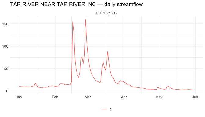
edr_plot() is a small ggplot wrapper for the tidy tibble:

edr_plot(df_jan_may) +
  ggtitle(paste0(example_name, " — daily streamflow"))

plot of chunk plot-one-gauge

If you already know the station IDs, the public batch helper performs the same bounded per-station workflow without discovering or parallelizing anything:

all_streamflow <- edr_location_batch(
  usgs, "daily-edr",
  location_id    = gauges$id,
  parameter_name = "00060",
  limit           = 200,
  max_requests    = nrow(gauges),
  on_error        = "collect",
  progress        = FALSE
)

all_streamflow$requests
all_streamflow$data
all_streamflow$errors

USGS beta currently ignores datetime on these individual location queries and returns the latest records. Do not add chunk here expecting historical windows: chunking is intended for EDR implementations that honor the requested interval.

4. Map every gauge with per-station popups

edr_explore() does the per-station loop and hands the results to edr_map() in one call. Each marker becomes an inline plot + CSV download for that gauge.

m <- edr_explore(
  usgs, "daily-edr",
  bbox           = piedmont_bbox,
  parameter_name = "00060",
  record_limit   = 200,                 # ~6 months of daily values per station
  popup          = "plot+csv",
  label_col      = "monitoring_location_name",
  quiet          = TRUE
)

Print m in an interactive R session to open the map. Click any blue marker to open the popup; its Jan–May 2026 streamflow plot is inline, and the “Download CSV” link delivers that gauge’s series.

To write the same map to a standalone HTML file, use edr_save_html():

edr_save_html(m, "piedmont-streamgages.html")

A few things worth knowing about the USGS endpoint

daily-edr only advertises the locations query. The other EDR verbs (cube, area, position, …) return HTTP errors. The per-station fallback works fine for tens of gauges; for hundreds consider pre-filtering aggressively with bbox =.
datetime is not honoured on /locations/{id} requests – the server returns the latest limit records regardless. Pass enough limit to cover your window, then filter client-side.
The station id format is "USGS-<NWIS-id>". The bare NWIS id ("02087500") doesn’t work; pass the full "USGS-..." form, which is what edr_locations() returns in its id column.
The 44-column attribute table on gauges carries a lot of useful metadata (drainage_area, state_name, hydrologic_unit_code, altitude, …). Use it to filter or label before mapping.
Pass label_col = "monitoring_location_name" to edr_map() so popup titles read “BUFFALO CREEK NEAR FALLS, NC” instead of the raw USGS-02087183 id.